On 11 May 2021, ECMWF implemented a substantial upgrade of its Integrated Forecasting System (IFS). As with almost all upgrades, this involved contributions from many teams within the Centre. IFS Cycle 47r2 includes changes to the forecast model, but not to the data assimilation system. The upgrade is neutral for the medium-range deterministic high-resolution (HRES) forecast but brings benefits to the medium- and extended-range ensemble forecasts (ENS). Cycle 47r2 is the culmination of two strands of work:
- A change from double precision to single precision in HRES and ENS forecasts
- An increase in the number of model levels from 91 to 137 in ENS forecasts
Forecast model
Previous versions of the IFS have used ‘double precision’, where each number is stored using 64 bits of memory. This is often more accurate than required when we consider observational errors and model approximations. Single precision, in which each number is stored with 32 bits of memory, offers the prospect of freeing up memory and, importantly, increasing processing speeds. Single precision of the IFS started as a research project in collaboration with the University of Oxford and as part of the OpenIFS effort. Similar lines of research were pursued in the COSMO (Consortium for Small-scale Modelling) model. It then became a collaborative project across many ECMWF teams. With more people working on the project, forecast skill became increasingly neutral over time with respect to double precision, up to a point where it could be incorporated into our operational forecasts. This allows computational savings to be made which can be used to achieve skill improvements. Figure 1 shows the computational changes to the ensemble forecast. Faster core processing (green circles) of single-precision data permits a 50% increase in ENS model levels from 91 to 137. Even with this increase in levels, data transferred (red arrows) between the memory on each node (yellow boxes) is reduced because it is now in single precision.

Double precision is still used throughout the data assimilation process, and some calculations in the forecast do still require double precision. The most expensive of those, such as the calculation of the associated Legendre polynomials and the finite-element integral operators of the vertical discretisation, are only done once and are not repeated during time-stepping. Hence, there is minimal impact on computational efficiency. Further detailed experimentation helped us to identify a few other calculations in parts of dynamics and physics and the stochastic physics perturbations that need to be secured with double precision. However, those also represent a very small part of the total computational load. Note also that GRIB encoding is unchanged, so archived files remain the same size.
The change to 137 levels brings us one step closer to a more seamless ensemble data assimilation and forecasting system. The need for vertical interpolation when generating ensemble initial conditions is now greatly reduced as the ensemble of data assimilations (EDA) is already run with 137 levels. The consistency with the HRES vertical resolution should also aid the evaluation process of future cycles. Technical changes to the ensemble include the calculation of singular vector perturbations with 137 levels.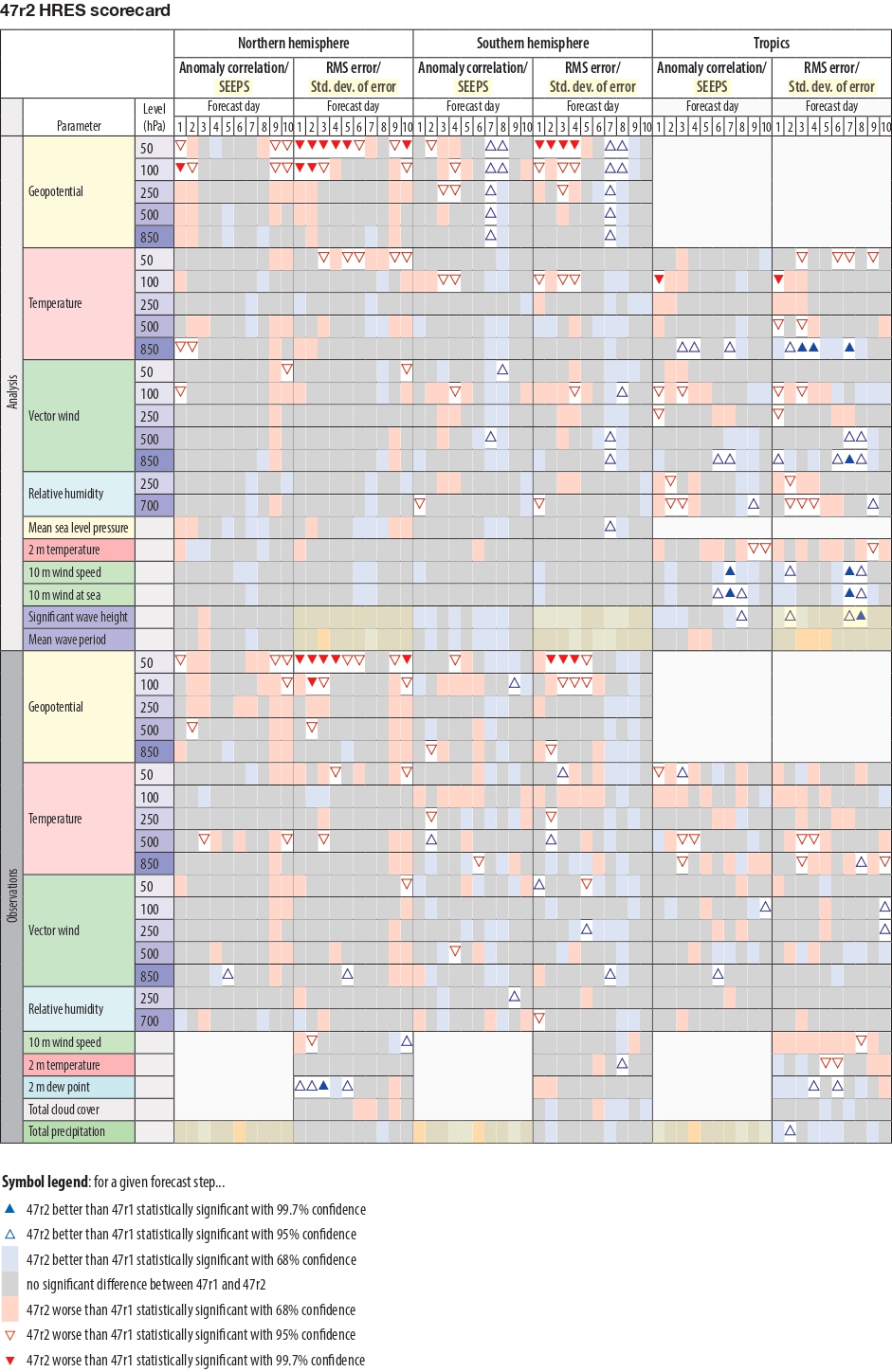
Impact on medium- and extended-range forecasts
The goal for the implementation of single precision was neutrality in HRES scores, together with major computational cost savings. Neutrality would be demonstrated in an HRES scorecard (Figure 2) with approximately a third of the boxes being grey, a third red and a third blue, and with little more than 5% of the red and blue boxes being statistically significant at the 5% significance level (indicated by triangles). As can be seen in Figure 2, this has largely been achieved. A possible exception is a degradation (typically less than 1%) in stratospheric extratropical geopotential height scores.
The neutrality for the HRES is illustrated in Figure 3 by track forecasts of Hurricane Laura. While agreement cannot be perfect for a chaotic system, the medium-range track differences between single and double precision are much smaller than the spread of the ensemble, which represents the impacts of initial and model uncertainty. More generally, the impact of single precision on HRES tropical cyclone track and intensity scores is neutral.

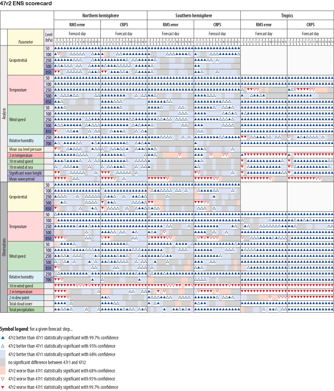
The increase in vertical resolution from 91 to 137 levels has been introduced to all ENS forecasts in the medium to the extended range. The ENS scorecard is shown in Figure 4. The change leads to statistically significant improvements to many ENS scores of about 0.5–2% throughout most of the free atmosphere. Stratospheric temperature scores are greatly improved, typically by 5–20%. This is, among other things, due to a weaker growth of temperature biases because the ENS can better resolve gravity waves in the vertical. Figure 5 shows this improvement at day 10, but it persists into the extended range. The mean cooling difference below 600 hPa (Figure 5 bottom panel) acts to decrease the warm bias around 850 hPa. It improves tropical medium-range scores at that level by over 6%. It does also slightly increase the tropical near-surface cool bias, and this is reflected in the 2‑metre temperature scores in Figure 4, which are degraded by up to 1% by day 14. Ten-metre wind scores are also slightly degraded by 0.1–0.3%.
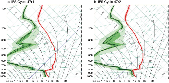
The extra levels mean that sharper inversions can be resolved. For example, the ensemble vertical profile product now uses 34 model levels below 700 hPa instead of the previous 22. The Cycle 47r2 test profile in Figure 6, which uses the new mapping of model levels, shows a slightly sharper thermal inversion at around 850 hPa than the Cycle 47r1 profile. Users will need to ensure that they extract the correct model levels when creating their own forecast products.
Tropical cyclones show reduced intensity errors (see Figure 7a). This is largely associated with reduced bias. There is a mean reduction of about 2 hPa in central pressure in the medium range, increased spread, and improved reliability as measured by the spread-error agreement. The cycle is neutral in terms of track errors (Figure 7b). Along with the increased tropical cyclone intensity, other tropical activity is increased: calculating anomalies from the operational extended-range re‑forecasts may be advisable.
A key source of sub-seasonal predictability is the Madden–Julian Oscillation (MJO). Out to the extended range, the amplitude of the MJO is better sustained: the amplitude loss by day 15 is now about 15% rather than the previous value of about 20% (Figure 8). There is also an increase in MJO spread, improved reliability and better scores. Changes come mostly from improvements in tropical zonal winds at 200 hPa.

Forecast outputs
More frequent tropical cyclone track updates are now available with the inclusion of forecasts from 6 and 18 UTC initial times, alongside those of the 0 and 12 UTC forecasts. More snowfall Extreme Forecast Index (EFI) and Shift of Tails (SOT) products are now available with the inclusion of 3-, 5-, 10- and 15‑day accumulation periods, in addition to the previous 1‑day accumulations. A selection of new specialist climatological model parameters includes some which describe the characteristics of topographic features smaller than the model grid box, some which are used within radiation calculations, and the ‘Logarithm of surface roughness length for heat’.


Summary
The change to single precision in forecast mode for the HRES and ENS systems has freed up computing resources to be used to enhance forecast skill. In IFS Cycle 47r2, the choice has been made to use these resources to make the model levels used in the ENS match those of the EDA and HRES systems. This represents an important step within ECMWF’s ten‐year Strategy 2021–2030, which highlights “work towards a seamless integration from the ensemble of data assimilations to the ensemble forecast system”. The fact that the ENS and HRES now have the same model levels should also facilitate future cycle development. The new cycle increases ENS forecast skill by typically 0.5–2% in the free atmosphere, but by 5–20% for stratospheric temperatures at 50 hPa and by 6% in the tropical troposphere. It also intensifies tropical cyclones, thus reducing intensity errors and improving reliability, and it helps to better sustain the amplitude of the Madden–Julian Oscillation into the extended range.
Further reading
Lang, S.T.K., A. Dawson, M. Diamantakis, P. Dueben, S. Hatfield, M. Leutbecher et al.: More Accuracy with Less Precision, submitted to QJRMS.
Polichtchouk, I., T. Stockdale, P. Bechtold, M. Diamantakis, S. Malardel, I. Sandu et al.: 2019. Control on stratospheric temperature in IFS: resolution and vertical advection. ECMWF Technical Memorandum No. 847.
Váňa, F., P. Düben, S. Lang, T. Palmer, M. Leutbecher, D. Salmond et al.: 2017. Single Precision in Weather Forecasting Models: An Evaluation with the IFS. Monthly Weather Review, 145(2), 495–502.